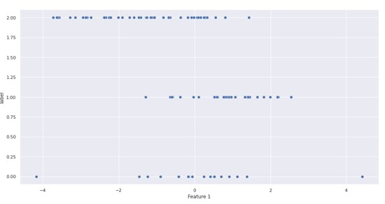
In this Tutorial we will learn how to create simulated data from classification in Python. Introduction Simulated data can be defined as any data not representing the real phenomenon but which is generated synthetically using parameters and constraints. W...
In this Tutorial we will learn how to create simulated data from classification in Python.
Simulated data can be defined as any data not representing the real phenomenon but which is generated synthetically using parameters and constraints.
Sometimes while prototyping a particular algorithm in Machine Learning or Deep Learning we generally face a scarcity of good real-world data which can be useful to us. Sometimes there is no such data **ailable for a given task. In such scenarios, we may need synthetically generated data. This data can also be from Lab Simulations.
Mostly represents data as it might be in the real form
Contains less variation of noise, so can be considered an ideal dataset
Useful for quick prototyping and POCs
In this demonstration, we are going to use sci-ki learn to generate simulated data.
Feature Dataframe:
   Feature 1    Feature 2    Feature 3    Feature 4    Feature 5    Feature 6 \
0  0.849715     -0.381343    0.650106     -1.439747    -0.442026    0.785891
1  1.841786     0.912779     2.090686     -2.220130    -0.744132    -0.116817
2  -0.915034    -3.324696    -2.613417    0.852612     -3.908363    4.352266
3  1.305116     -1.582905    -0.797318    -0.943912    -1.753893    1.721998
4  0.894486     -0.130399    -0.968311    0.989773     -0.987330    -0.296457
   Feature 7    Feature 8    Feature 9    Feature 10 label
0  0.119725     1.156633     0.794226     0.511587   2
1  -0.064624    2.311732     0.178347     1.294978   1
2  3.038898     -2.273558    4.194868     2.693096   2
3  0.817046     0.577196     2.651006     1.826657   2
4 -0.280331     0.096983     1.227921     0.909471   2

Another method is using the Faker python library. Let's see through the below example. Installing the Faker library
id	name	address	\
	7.0	Monique Rodriguez	481 Rebecca Landing Suite 727\nDominiquefurt, ...
	4.0	Elizabeth Johnson	62492 Zimmerman Crest Apt. 047\nPort Jerome, W...
	18.0	Max Rangel	4379 Obrien Curve\nD**istown, IA 02341
	31.0	Tammie Kent	4866 Angela Turnpike Apt. 658\nNorth Sheilabor...
	42.0	James Johnston	26827 Jeremiah Alley\nFreystad, SC 86902
	21.0	Shawn Robles	137 Jessica Ridges Apt. 436\nWilliamburgh, AZ ...
	13.0	Stephen Hodges	Unit 9799 Box 0625\nDPO AA 94415
	91.0	Eric Lewis PhD	4711 Nicholas Loaf\nWest Lisa, UT 28944
	68.0	Matthew Munoz	37836 White Crest\nGonzalezport, NC 75320
	34.0	Lawrence Anderson	76712 Garza Mills Apt. 751\nPort Penny, CT 43042

latitude		longitude	target 0	60.574796	109.367770		clerk
1	84.7225155	-167.216393	dr.
2	82.598649	62.961322	surgeon
3	26.9617205	89.333171	doctor
4	-37.1740195	-140.766121	dr.
5	-40.8904645	28.820918	clerk
6	88.809220	76.442779	dr.
7	35.728143	178.729120	doctor
8	-16.5669945	126.686740	dr.
9	-49.271970	160.737754	clerk
Simulated data is highly useful in day-to-day Machine Learning applications for prototyping or small POCs. There are some handy tools in Python which make this highly simple to create simulated data within a few lines of code.